Lab 4

Getting started

Use these steps to navigate to the STA101 version of RStudio using the Duke Container Manager;
Use these steps to download all of the lab 4 files from our Canvas page, upload them to your RStudio files, and move them into an appropriately named folder (lab-4, for instance);
Once lab-4.qmd is where it needs to be, open it, and verify that you can click the “Render” button in RStudio and get a PDF file. See this answer on Ed if you want more guidance here;
Now proceed to complete the exercises in this lab.

Pointers

For all visualizations you create, be sure to include informative titles for the plot, axes, and legend;
Respond in complete sentences as much as possible;
Be sure to observe good code style:
- There is a line break after each |> in a pipeline or + in a ggplot;
- There are spaces around = signs;
- There is a space after each ,;
- Code is properly indented;
- Code doesn’t exceed 80 characters in each line, longer lines of code are spread across multiple lines with appropriately placed line breaks (so in the rendered PDF, your code shouldn’t run off the page);
- Code chunks are labeled, informatively and without spaces.

Packages

library(tidyverse) 
library(tidymodels)

Part 1: Do you even lift?

Today, we will be working with data from www.openpowerlifting.org. This data was sourced from Tidy Tuesday and contains international powerlifting records at various meets. At each meet, each lifter gets three attempts at lifting max weight on three lifts: the bench press, squat and deadlift.

ipf <- read_csv("data/ipf.csv")

Note

Recall that you may have to adjust the file path to match how you have organized your files and folders.

The data dictionary for this dataset from TidyTuesday is reproduced below:

variable	description
`name`	Individual lifter name
`sex`	Binary gender (M/F)
`event`	The type of competition that the lifter entered. Values are as follows: SBD: Squat-Bench-Deadlift, also commonly called “Full Power” BD: Bench-Deadlift, also commonly called “Ironman” or “Push-Pull” SD: Squat-Deadlift, very uncommon SB: Squat-Bench, very uncommon S: Squat-only B: Bench-only D: Deadlift-only
`equipment`	The equipment category under which the lifts were performed. Values are as follows: Raw: Bare knees or knee sleeves Wraps: Knee wraps were allowed Single-ply: Equipped, single-ply suits Multi-ply: Equipped, multi-ply suits (includes Double-ply) Straps: Allowed straps on the deadlift (used mostly for exhibitions, not real meets)
`age`	The age of the lifter on the start date of the meet, if known.
`age_class`	The age class in which the filter falls, for example `40-45`
`division`	Free-form UTF-8 text describing the division of competition, like `Open` or `Juniors 20-23` or `Professional`.
`bodyweight_kg`	The recorded bodyweight of the lifter at the time of competition, to two decimal places.
`weight_class_kg`	The weight class in which the lifter competed, to two decimal places. Weight classes can be specified as a maximum or as a minimum. Maximums are specified by just the number, for example `90` means “up to (and including) 90kg.” minimums are specified by a `+` to the right of the number, for example `90+` means “above (and excluding) 90kg.”
`best3squat_kg`	Maximum of the first three successful attempts for the lift. Rarely may be negative: that is used by some federations to report the lowest weight the lifter attempted and failed.
`best3bench_kg`	Maximum of the first three successful attempts for the lift. Rarely may be negative: that is used by some federations to report the lowest weight the lifter attempted and failed.
`best3deadlift_kg`	Maximum of the first three successful attempts for the lift. Rarely may be negative: that is used by some federations to report the lowest weight the lifter attempted and failed.
`place`	The recorded place of the lifter in the given division at the end of the meet. Values are as follows: Positive number: the place the lifter came in. G: Guest lifter. The lifter succeeded, but wasn’t eligible for awards. DQ: Disqualified. Note that DQ could be for procedural reasons, not just failed attempts. DD: Doping Disqualification. The lifter failed a drug test. NS: No-Show. The lifter did not show up on the meet day.
`date`	ISO 8601 Date of the event
`federation`	The federation that hosted the meet. (limited to IPF for this data subset)
`meet_name`	The name of the meet. The name is defined to never include the year or the federation. For example, the meet officially called `2019 USAPL Raw National Championships` would have the MeetName `Raw National Championshps`.

For all of the following exercises, you should include units on axes labels, e.g. “Bench press (lbs)” or “Bench press (kg)”. “Age (years)” etc. This is good practice.

Exercise 1

Let’s begin by taking a look at the squat lifting records.

To begin, remove any observations that are negative for squat. Next, create a new column called best3_squat_lbs that converts the record from kg to lbs (you may have to Google the conversion). Save your data frame as ipf_squat. Report the number of rows and columns of this new data frame.

Hint

First, you’re taking a dataset and filtering it for certain records, and then you’re mutate-ing that dataset to gain a new column, and you’re assigning the resulting dataset to a new object called ipf_squat.

Exercise 2

Using ipf_squat from the previous exercise, create a scatter plot to investigate the relationship between squat (in lbs) and age. Age should be on the x-axis. Adjust the alpha level of your points to get a better sense of the density of the data. Add a linear trend-line. Be sure to label all axes and give the plot a title. Comment on what you observe.

Exercise 3

Write down the linear model to predict lift squat lbs from age in \(x\), \(y\), \(\beta\) notation. What is \(x\)? What is \(y\)? Next, fit the linear model, and save it as age_fit. Re-write your previous equation replacing \(\beta\) with the numeric estimates. This is called the “fitted” linear model. Interpret each estimate of \(\beta\). Are the interpretations sensible?

Exercise 4

Building on your ipf_squat data frame, create a new column called age2 that takes the age of each lifter and squares it. Save it to your data frame ipf_squat. Next, plot squat in lbs vs age2 and add a linear best fit line. Does this model look like it fits the data better?

Hint

To raise a value to a power, use ^ in R, e.g.: 2 ^ 2 gives you 4, 2 ^ 3 gives you 8, etc.

Exercise 5

One metric to assess the fit of a model is \(R^2\). Fit the age\(^2\) model and save the object as age2_fit. Compare \(R^2\) of the age\(^2\) model to the \(R^2\) of the model from Exercise 3. Which has a higher \(R^2\)?

Exercise 6

Next, let’s turn our attention to dead lifting records.

Recreate the plot below. Make sure axes and title labels are exactly matching, including spelling, capitalization, etc. Based on the plot below, which impacts deadlift weight more, age category or sex?

Hint 1

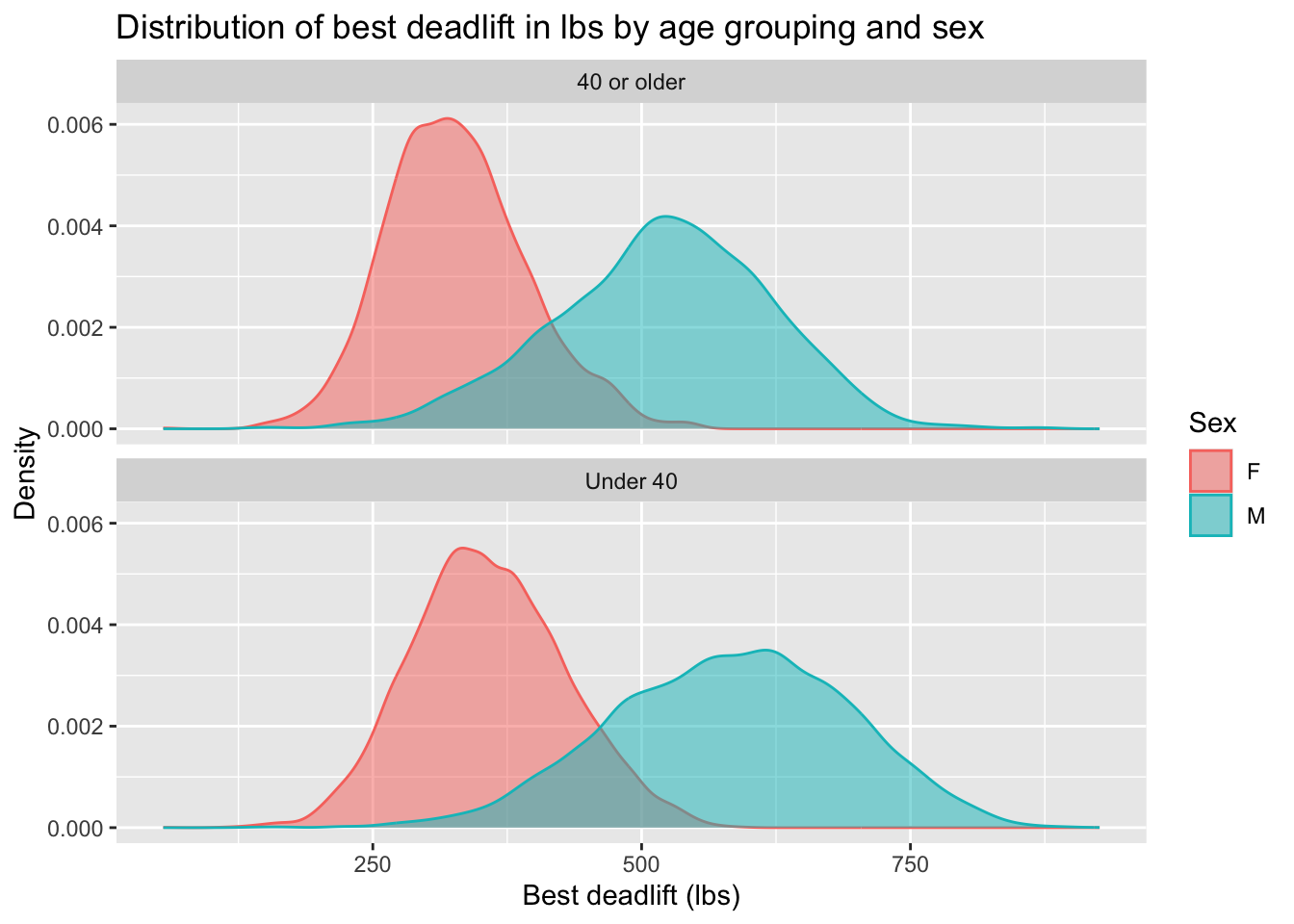
You will need to create a couple of new columns. One to classify age appropriately and one to convert best3deadlift_kg to the plotted units (lbs). Notice that there are no negative deadlift values on the x-axis.

Hint 2

These plots are called density plots. It’s just a smoothed out version of a histogram, and like the histogram it lets you visualize the distribution (center, spread, skew, etc) of a dataset. The geom_... that creates density plots is geom_density. Try it out!

Exercise 7

Finally, let’s turn our attention to bench press records.

To begin, remove any observations that are negative for bench press, create two new columns: best3bench_lbs and bodyweight_lbs. Save the result in a new data frame called ipf_bench.

Then, create a scatter plot to investigate the relationship between best bench press (in lbs) and the lifter’s bodyweight (in lbs). Bodyweight should be on the x-axis. Add a linear trend-line. Be sure to label all axes and give the plot a title. Comment on what you observe.

Exercise 8

Fit the linear model displayed in the previous exercise and write down the fitted model equation only, replacing \(\hat{\beta}\)s with their fitted estimates. Interpret the \(\hat{\beta}\)s (intercept and slope). Report \(R^2\). Is body weight an important predictor of bench press ability? Why or why not?

Part 2: IMS Exercises

The exercises in this section do not require code. Make sure to answer the questions in full sentences.

Exercise 9

IMS - Chapter 7 exercises, #18: Over-under, II.

Exercise 10

IMS - Chapter 7 exercises, #24: Cats weights.

Lastly

Recommend some music for us to listen to while we grade this.

Wrap up

Submitting

Important

Before you proceed, first, make sure that you have updated the document YAML with your name! Then, render your document one last time, for good measure.

To submit your assignment to Gradescope:

Go to your Files pane and check the box next to the PDF output of your document (lab-4.pdf).
Then, in the Files pane, go to More > Export. This will download the PDF file to your computer. Save it somewhere you can easily locate, e.g., your Downloads folder or your Desktop.
Go to the course Canvas page and click on Gradescope and then click on the assignment. You’ll be prompted to submit it.
Mark the pages associated with each exercise. All of the papers of your lab should be associated with at least one question (i.e., should be “checked”).

Warning

If you fail to mark the pages associated with an exercise, that exercise won’t be graded. This means, if you fail to mark the pages for all exercises, you will receive a 0 on the assignment. The TAs can’t mark your pages for you, and for them to be able to grade, you must mark them.

Grading

Exercise	Points
Exercise 1	3
Exercise 2	5
Exercise 3	5
Exercise 4	5
Exercise 5	5
Exercise 6	8
Exercise 7	6
Exercise 8	7
Exercise 9	1
Exercise 10	5
Total	50