Confidence intervals with the bootstrap

A $100\times(1-\alpha)\%$ confidence interval is an interval $(L_n,\,U_n)$ that contains the true value $\theta$ of some quantity of interest with high probability across repeated sampling. In order to approximate such an interval in general, we use the bootstrap to approximate the sampling distribution of an estimator $\hat{\theta}$, and then we use the quantiles of that boostrap distribution to determine the bounds of our interval.

This primer leads you down the path of least resistance to…doing all that.

Setup

Load our packages as usual:

library(tidyverse) 
library(tidymodels)

Next, consider this lil’ dataset:

abb <- read_csv("asheville.csv")

abb

# A tibble: 50 × 1
     ppg
   <dbl>
 1  48  
 2  40  
 3  99  
 4  13  
 5  55  
 6  75  
 7  74  
 8 169  
 9  56.2
10  74.5
# ℹ 40 more rows

These are data on the price per guest in USD (ppg) for a random sample of fifty Airbnb listings in 2020 for Asheville, NC. We are going to use these data to investigate what we would be expected to pay for an Airbnb in in Asheville, NC in June 2020. Here is what the data look like:

ggplot(abb, aes(x = ppg)) + 
  geom_histogram() +
  labs(x = "Price per guest ($)")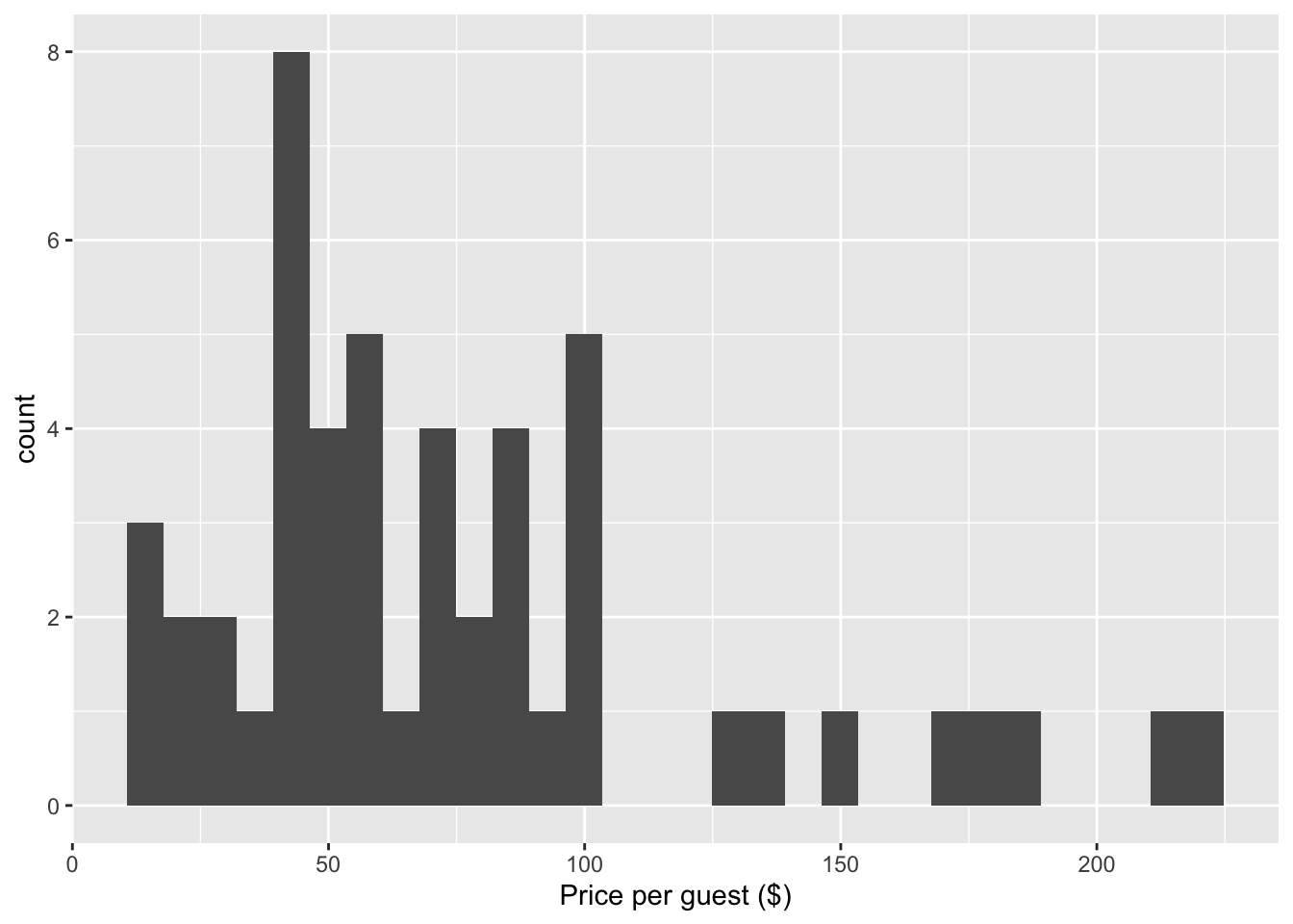

To answer the question “what was the typical or expected price,” we can calculate a point estimate like the sample mean or sample median:

abb |> 
  summarize(mean = mean(ppg),
            median = median(ppg))

# A tibble: 1 × 2
   mean median
  <dbl>  <dbl>
1  76.6   62.5

In this case they disagree quite a bit, which in general is something you should think about, but for the purposes of this primer, we will set the issue aside and focus just on the sample mean as our estimate.

Approximating the sampling distribution of the mean with the bootstrap

The sampling distribution of the mean refers to the random variation we would observe in our mean estimate if we recomputed it based on many different hypothetical samples from the population (June 2020 Airbnb listings in Asheville, in this case). Unfortunately, we do not have many different samples from this population. We only have one sample. But if that sample is a decent approximation to the population (debateable, in this case), we can randomly generate different hypothetical samples from our sample (resamples), calculate a different mean for each, and look at the variation in those estimates.

This is dirty work, but thankfully the computer handles it with aplomb:

set.seed(8675309) 

boot_dist_abb <- abb |>
  specify(response = ppg) |>
  generate(reps = 5000, type = "bootstrap") |>
  calculate(stat = "mean")

boot_dist_abb

Response: ppg (numeric)
# A tibble: 5,000 × 2
   replicate  stat
       <int> <dbl>
 1         1  70.8
 2         2  66.2
 3         3  72.8
 4         4  73.1
 5         5  76.4
 6         6  80.1
 7         7  80.4
 8         8  69.1
 9         9  91.7
10        10  74.1
# ℹ 4,990 more rows

The code works like this:

specify(response = ppg): this is a bookkeeping step where we tell the computer which column in our data frame we are studying. It’s simple in this case because there is only one;
generate(reps = 5000, type = "bootstrap"): this generates 5000 bootstrap datasets. In general, we want the numbers of replicates/repetitions to be large enough for the approximation to be good, but not so large that it takes a while to run or hogs all the memory on our computer. For the small applications in our course, 1000 - 5000 replicates should suffice;
calculate(stat = "mean"): once we have the bootstrap datasets, we need to calculate the value of our desired statistic for each one. The variation in these estimates captures what we mean by “sampling uncertainty.” For these Airbnb data, the statistic we care about is the sample average or mean, so that’s what we ask for, but there are several options: “mean”, “median”, “sd”, “prop”, “diff in means”, “diff in props”, and so on.

ggplot(boot_dist_abb, aes(x = stat)) + 
  geom_histogram()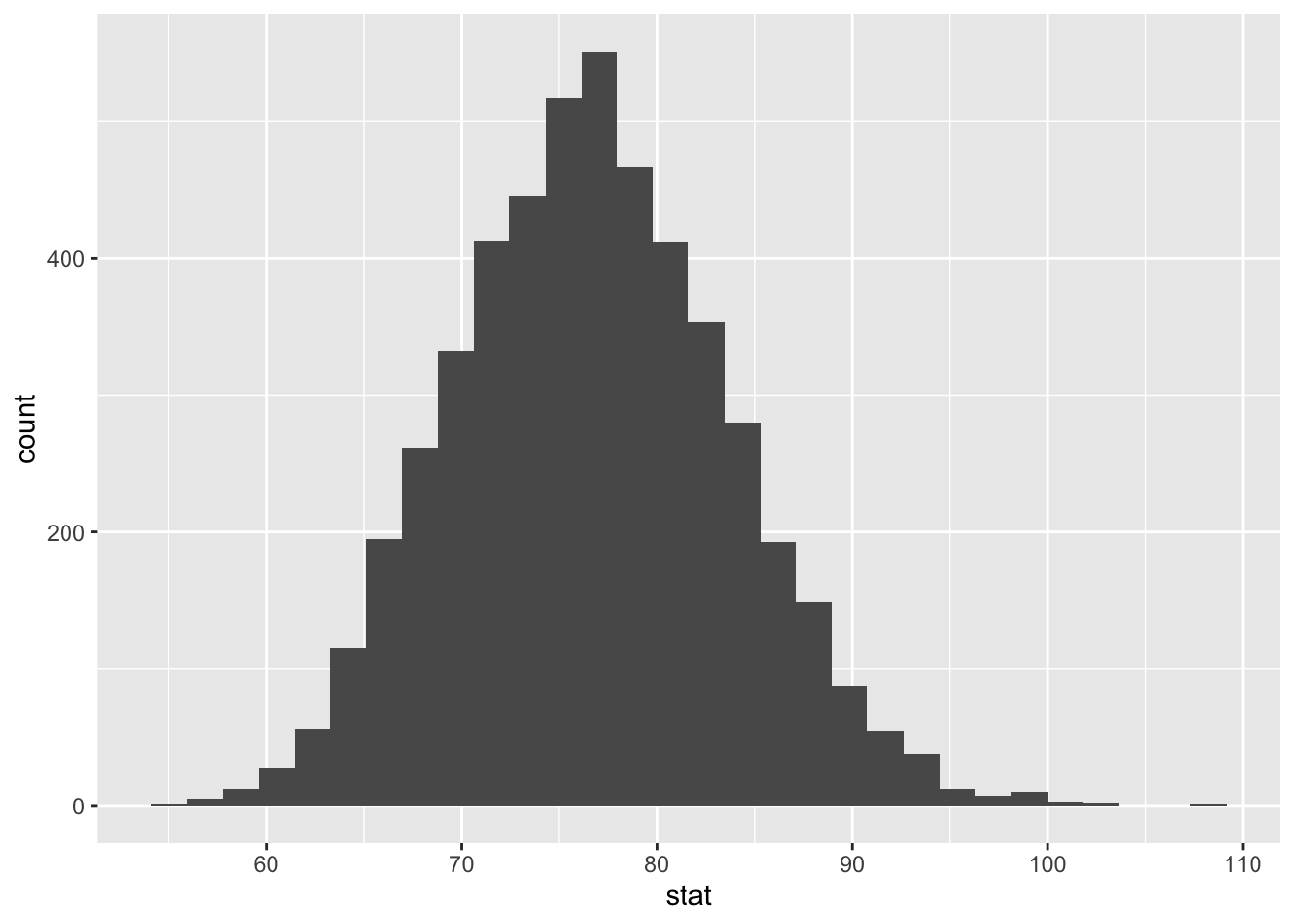

Calculating an approximate confidence interval

Armed with our bootstrap sample of different means, we can calculate a 95% confidence interval using the quantile function:

boot_dist_abb |>
  summarize(
    lower = quantile(stat, 0.025),
    upper = quantile(stat, 0.975)
  )

# A tibble: 1 × 2
  lower upper
  <dbl> <dbl>
1  63.8  90.9

Alternatively, we can use this nifty command which gives the same numbers:

ci_95_abb <- boot_dist_abb |>
  get_confidence_interval(
    point_estimate = mean(abb$ppg), 
    level = 0.95
  )
ci_95_abb

# A tibble: 1 × 2
  lower_ci upper_ci
     <dbl>    <dbl>
1     63.8     90.9

Lastly, we can summarize it all with a picture:

visualize(boot_dist_abb) +
  shade_confidence_interval(ci_95_abb)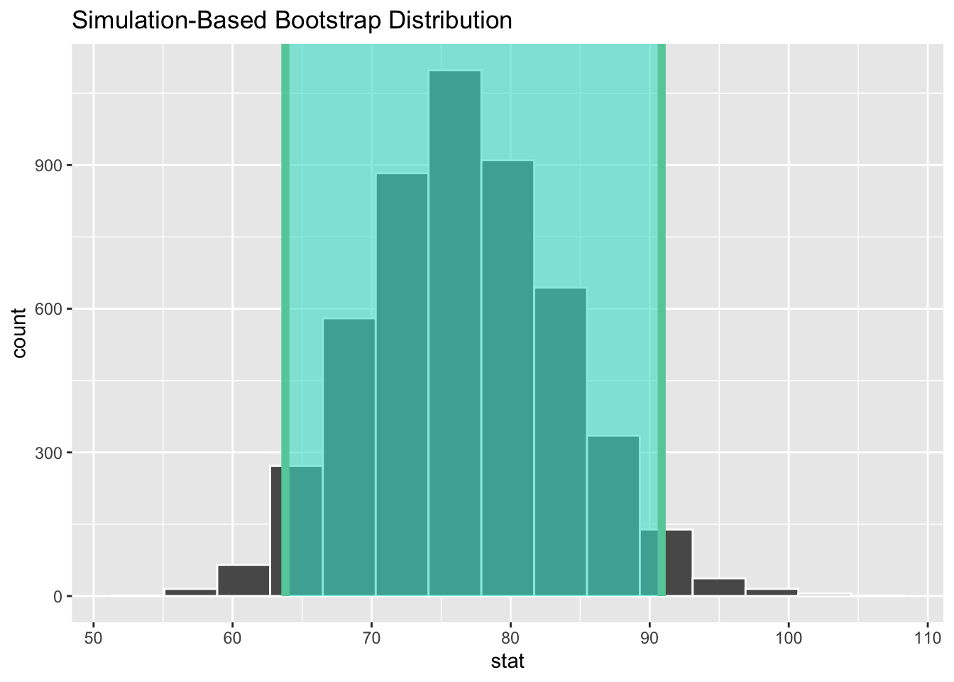

The correct language for interpreting our interval goes something like this:

We are 95% confident that the true mean price lies in between $65.55 and $88.45.

But what does “95% confident” actually mean? It refers to the reliability in repeated use of the method that was used to generate the interval. It does not say anything about the reliability of the specific interval (65.55, 88.45), which is a tad disappointing.

Think of it this way: if each day for 1000 days, we collected a new random sample of prices, and calculated a 95% confidence interval for each of those samples, approximately 950 of those 1000 intervals would contain the truth. That’s the sense in which the interval estimation method is 95% reliable. In practice however, we have one dataset and one interval. So how do we know if our interval is one of those lucky 950, or if we’re one of the 50 that went astray? Welcome to statistics, folks.