Simple linear regression

The simple linear regression model relates a predictor $x$ to a response $y$ via a linear function with error:

\[ y=\beta_0+\beta_1x+\varepsilon. \]

This primer leads you down the path of least resistance to fitting this model, creating a scatterplot with the best fit line added to it, and producing a table with the coefficient estimates ($\hat{\beta}_0,\,\hat{\beta}_1$).

Setup

The commands for working with linear regressions are in the tidymodels package, so load that:

library(tidyverse) 
library(tidymodels)

Next, we need something to model, so let us load in a data set. We will consider this data set on the stock price of Microsoft and Apple (introduced during Lecture 6 on 9/12/2024):

stocks <- read_csv("stocks.csv")

Note

Recalling the information here, be prepared to adjust the file path to match how you have organized your files and folders.

To keep things simple, we’ll work with a subset of the data, stock prices in January 2020.

stocks_jan2020 <- stocks |>
  filter(month(date) == 1 & year(date) == 2020)

Plotting the least squares regression line (“line of best fit”)

This chunk of code creates a scatter plot of the Microsoft and Apple opening stock prices on the various trading days of January 2020, and it adds the line of best fit:

ggplot(stocks_jan2020, aes(x = MSFT.Open, y = AAPL.Open)) +
  geom_point() + 
  geom_smooth(method = "lm", se = FALSE, color = "red") +
  labs(
    title = "Daily stock price data",
    subtitle = "January 2020",
    x = "Microsoft opening price",
    y = "Apple opening price"
  )

`geom_smooth()` using formula = 'y ~ x'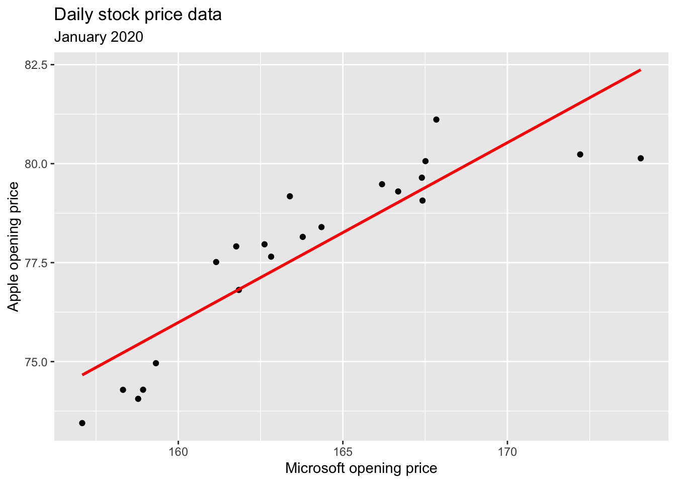

So, all we have to do is add a new geom_WHAT layer to a scatterplot to add the line. This is what geom_smooth is doing. If you set se = TRUE, you get the band indicating the margin of error. Try it out!

What are the coefficient estimates?

This code will give you a table with the estimates:

stock_fit <- linear_reg() |>
  fit(AAPL.Open ~ MSFT.Open, data = stocks_jan2020)

tidy(stock_fit)

# A tibble: 2 × 5
  term        estimate std.error statistic      p.value
  <chr>          <dbl>     <dbl>     <dbl>        <dbl>
1 (Intercept)    3.31     8.87       0.373 0.713       
2 MSFT.Open      0.454    0.0541     8.40  0.0000000808

There is a lot going on in that table, and we will explore some of it later, but focus on the first column for now. This column gives the estimates $\hat{\beta}_0,\,\hat{\beta}_1$. The first row has the estimate $\hat{\beta}_0$ of the intercept, and the second row has the estimate $\hat{\beta}_1$ of the slope. So the fitted model here is: \[ \begin{align*} \widehat{\text{AAPL}}&=\hat{\beta}_0+\hat{\beta}_1{\text{MSFT}}\\ &\approx3.31+0.45\cdot{\text{MSFT}}. \end{align*} \] So

3.31 is the price you would predict for Apple stock if you knew Microsoft stock was opening at $0;
0.45 is the price increase in Apple stock that you would predict if Microsoft stock became more expensive by $1 (remember, slope = rise/run, so $\Delta\text{AAPL}/\Delta\text{MSFT}$ in this case).

The syntax in the fit commands is like fit(y ~ x). So the variable to the left of the ~ will be treated as the response variable ($y$), and the variable to the right will be treated as the predictor ($x$).