library(tidyverse)
library(openintro)The normal distribution
The normal distribution is the familiar bell curve. The central limit theorem says that the sampling distribution of a statistic (sample mean, proportion, difference, etc) looks more and more like a normal distribution the more data we have. This gives us permission to use a normal distribution to approximate the sampling distribution, and use the convenient properties of the bell curve to compute confidence intervals and hypothesis tests.
This primer introduces you to the basic commands for working with the normal distribution.
Load packages
The openintro package has tools for working with the normal distribution:
Example: bone density
Suppose the bone density of 65-year-old women is normally distributed with mean 809 \(mg/cm^3\) and standard deviation of 140 \(mg/cm^3\). For reference, here are the densities for three types of wood:
Plywood: 540 \(mg/cm^3\)
Pine: 600 \(mg/cm^3\)
Mahogany: 710 \(mg/cm^3\)
If \(X\) represents the bone density of 65-year-old women, then we can summarize the situation mathematically by writing:
\[ X \sim N(\mu = 809, \sigma = 140). \]
Let’s give all of the numbers above names and store them in the computer for later:
bone_density_mean <- 809
bone_density_sd <- 140

plywood <- 540
pine <- 600
mahogany <- 710
Plot the bell curve
This handy-dandy function plots a bell curve:
normTail(m = 0, s = 1)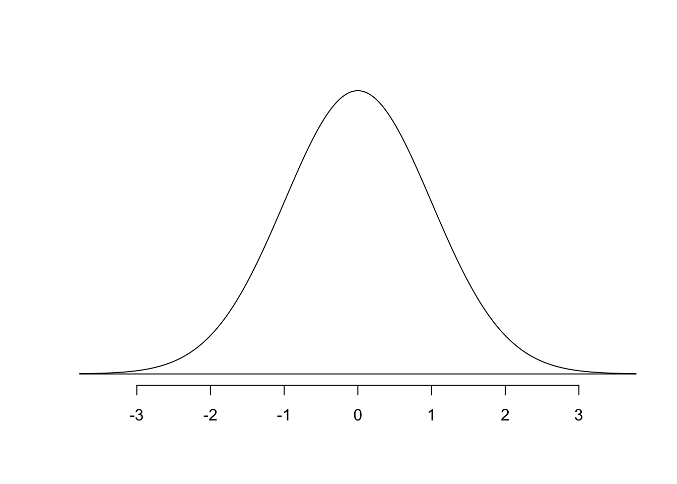
You can add several arguments to customize:
normTail(m = bone_density_mean,
         s = bone_density_sd,
         main = "Distribution of bone density of 65-year-old women",
         xlab = "mg/cm^3",
         xlim = c(200, 1400))
Compute quantiles under the normal distribution
The qnorm function computes the quantiles of a normal distribution. If we wanted the 50% quantile (AKA the median), we would say
qnorm(0.5, mean = 0, sd = 1)[1] 0In this case we just get back the mean, because the normal distribution is perfectly symmetric, and mean and median are equal for symmetric distributions.
If we wanted the inner quartile range (IQR) for a normal distribution, here it goes:
q25 <- qnorm(0.25, mean = 0, sd = 1)
q75 <- qnorm(0.75, mean = 0, sd = 1)

IQR <- q75 - q25
IQR
[1] 1.34898Compute and visualize probabilities under the normal distribution
What is the probability that a randomly selected 65-year-old woman has bones that are as or less dense than pine? If we add an L argument (for “lower”) to normTail, we can visualize the answer:
normTail(m = bone_density_mean, s = bone_density_sd, L = pine,
         main = "Distribution of bone density of 65-year-old women",
         xlab = "mg/cm^3",)
Notice how this may come in handy when we have to compute something like a \(p\)-value. In order to compute the probability (area) under the bell curve of being less than 600 \(mg/cm^3\), we can use the pnorm function:
pnorm(pine, mean = bone_density_mean, sd = bone_density_sd, lower.tail = TRUE)[1] 0.06773729Above, we asked about being under 600 in the distribution. But we could just have easily looked at being over 600 by adding a U argument (for “upper”):
normTail(m = bone_density_mean, s = bone_density_sd, U = pine,
         main = "Distribution of bone density of 65-year-old women",
         xlab = "mg/cm^3",)
To get the number, we change the lower.tail argument:
pnorm(pine, mean = bone_density_mean, sd = bone_density_sd, lower.tail = FALSE)[1] 0.9322627Notice that the probability of being at or below 600 is 6.77%. The probability of being above 600 is 93.23% That covers everything, so taken together you get 100%, which is the total area under the bell curve.