Model selection for logistic regression

Load packages and data

library(tidyverse)

── Attaching core tidyverse packages ──────────────────────── tidyverse 2.0.0 ──
✔ dplyr     1.1.4     ✔ readr     2.1.5
✔ forcats   1.0.0     ✔ stringr   1.5.1
✔ ggplot2   3.5.1     ✔ tibble    3.2.1
✔ lubridate 1.9.3     ✔ tidyr     1.3.1
✔ purrr     1.0.2     
── Conflicts ────────────────────────────────────────── tidyverse_conflicts() ──
✖ dplyr::filter() masks stats::filter()
✖ dplyr::lag()    masks stats::lag()
ℹ Use the conflicted package (<http://conflicted.r-lib.org/>) to force all conflicts to become errors

library(tidymodels)

── Attaching packages ────────────────────────────────────── tidymodels 1.2.0 ──
✔ broom        1.0.6     ✔ rsample      1.2.1
✔ dials        1.3.0     ✔ tune         1.2.1
✔ infer        1.0.7     ✔ workflows    1.1.4
✔ modeldata    1.4.0     ✔ workflowsets 1.1.0
✔ parsnip      1.2.1     ✔ yardstick    1.3.1
✔ recipes      1.1.0     
── Conflicts ───────────────────────────────────────── tidymodels_conflicts() ──
✖ scales::discard() masks purrr::discard()
✖ dplyr::filter()   masks stats::filter()
✖ recipes::fixed()  masks stringr::fixed()
✖ dplyr::lag()      masks stats::lag()
✖ yardstick::spec() masks readr::spec()
✖ recipes::step()   masks stats::step()
• Use suppressPackageStartupMessages() to eliminate package startup messages

library(forested)

glimpse(forested)

Rows: 7,107
Columns: 19
$ forested         <fct> Yes, Yes, No, Yes, Yes, Yes, Yes, Yes, Yes, Yes, Yes,…
$ year             <dbl> 2005, 2005, 2005, 2005, 2005, 2005, 2005, 2005, 2005,…
$ elevation        <dbl> 881, 113, 164, 299, 806, 736, 636, 224, 52, 2240, 104…
$ eastness         <dbl> 90, -25, -84, 93, 47, -27, -48, -65, -62, -67, 96, -4…
$ northness        <dbl> 43, 96, 53, 34, -88, -96, 87, -75, 78, -74, -26, 86, …
$ roughness        <dbl> 63, 30, 13, 6, 35, 53, 3, 9, 42, 99, 51, 190, 95, 212…
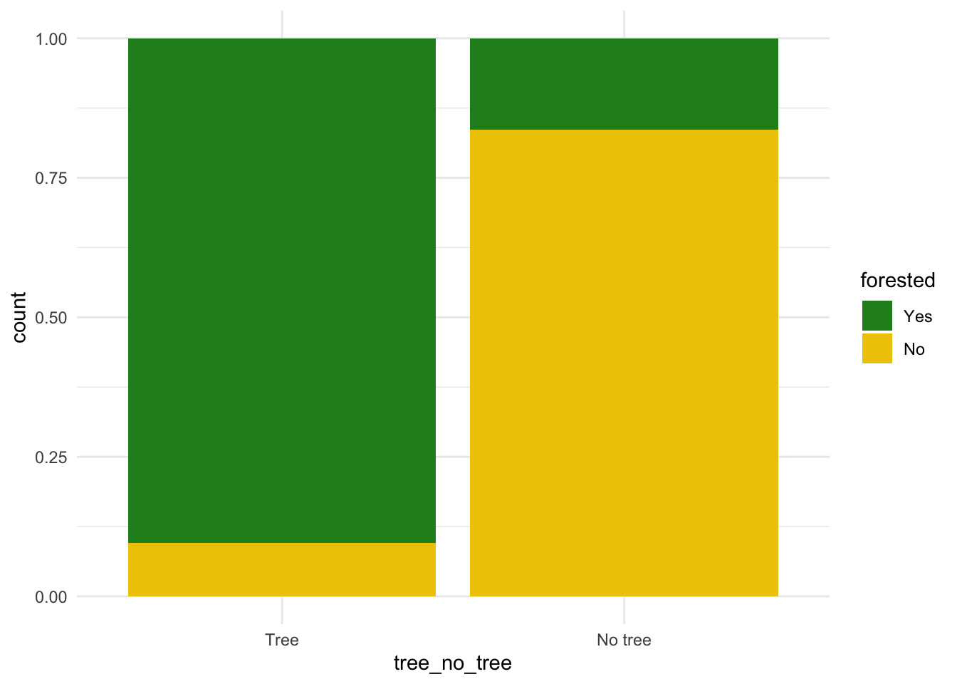
$ tree_no_tree     <fct> Tree, Tree, Tree, No tree, Tree, Tree, No tree, Tree,…
$ dew_temp         <dbl> 0.04, 6.40, 6.06, 4.43, 1.06, 1.35, 1.42, 6.39, 6.50,…
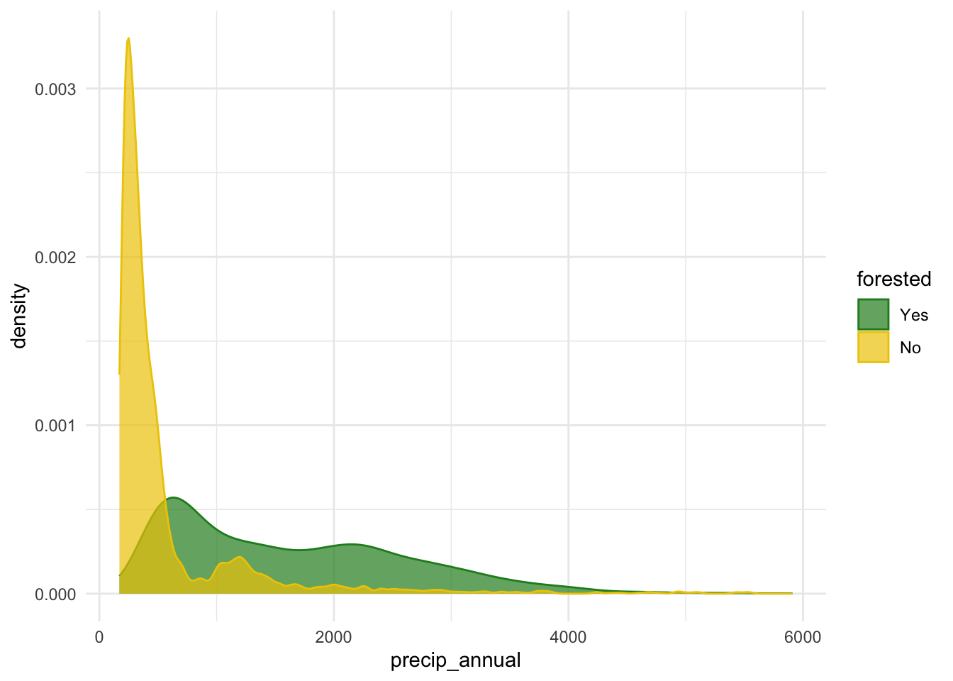
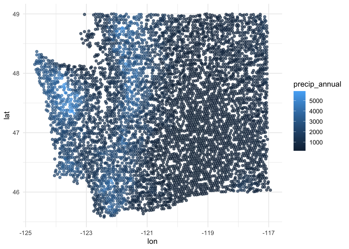
$ precip_annual    <dbl> 466, 1710, 1297, 2545, 609, 539, 702, 1195, 1312, 103…
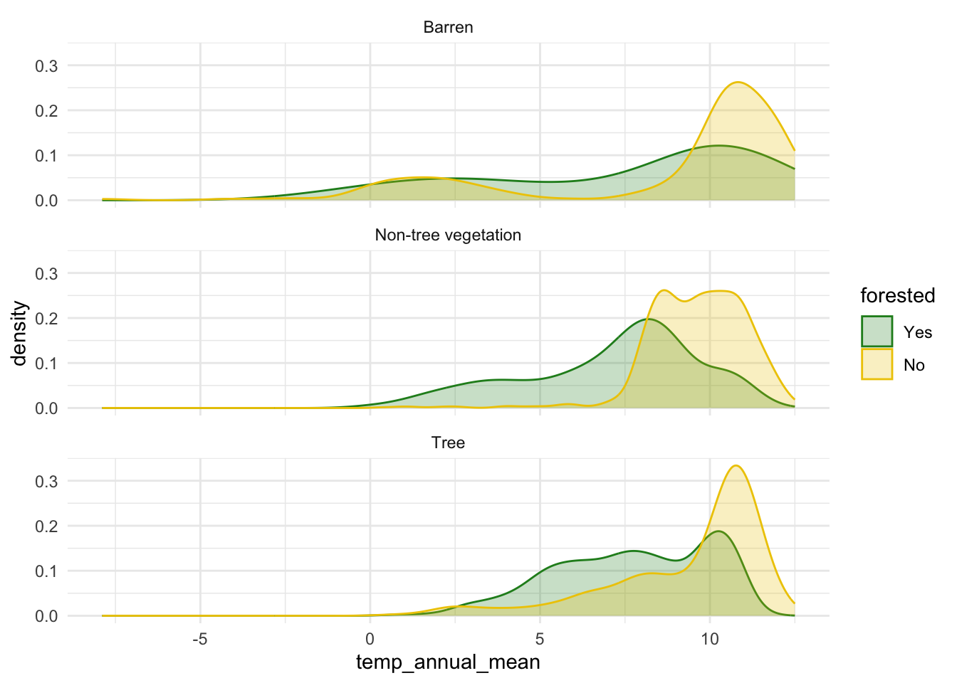
$ temp_annual_mean <dbl> 6.42, 10.64, 10.07, 9.86, 7.72, 7.89, 7.61, 10.45, 10…
$ temp_annual_min  <dbl> -8.32, 1.40, 0.19, -1.20, -5.98, -6.00, -5.76, 1.11, …
$ temp_annual_max  <dbl> 12.91, 15.84, 14.42, 15.78, 13.84, 14.66, 14.23, 15.3…
$ temp_january_min <dbl> -0.08, 5.44, 5.72, 3.95, 1.60, 1.12, 0.99, 5.54, 6.20…
$ vapor_min        <dbl> 78, 34, 49, 67, 114, 67, 67, 31, 60, 79, 172, 162, 70…
$ vapor_max        <dbl> 1194, 938, 754, 1164, 1254, 1331, 1275, 944, 892, 549…
$ canopy_cover     <dbl> 50, 79, 47, 42, 59, 36, 14, 27, 82, 12, 74, 66, 83, 6…
$ lon              <dbl> -118.6865, -123.0825, -122.3468, -121.9144, -117.8841…
$ lat              <dbl> 48.69537, 47.07991, 48.77132, 45.80776, 48.07396, 48.…
$ land_type        <fct> Tree, Tree, Tree, Tree, Tree, Tree, Non-tree vegetati…

Split data

set.seed(1234)
forested_split <- initial_split(forested)
forested_train <- training(forested_split)
forested_test <- testing(forested_split)

Exploratory data analysis

ggplot(forested_train, aes(x = precip_annual, fill = forested, color = forested)
  ) +
  geom_density(alpha = 0.7) +
  theme_minimal() + 
  scale_fill_manual(values = c("Yes" = "forestgreen", "No" = "gold2")) +
  scale_color_manual(values = c("Yes" = "forestgreen", "No" = "gold2"))

ggplot(forested_train, aes(x = tree_no_tree, fill = forested)) +
  geom_bar(position = "fill") +
  scale_fill_manual(values = c("Yes" = "forestgreen", "No" = "gold2")) +
  theme_minimal()

ggplot(
  forested_train,
  aes(x = temp_annual_mean, fill = forested, color = forested)
  ) +
  geom_density(alpha = 0.25) +
  scale_fill_manual(values = c("Yes" = "forestgreen", "No" = "gold2")) +
  scale_color_manual(values = c("Yes" = "forestgreen", "No" = "gold2")) +
  facet_wrap(~land_type, ncol = 1) +
  theme_minimal()

Crude map!

(What about coloring points by a numerical quantity?)

ggplot(forested_train, aes(x = lon, y = lat, color = precip_annual)) +
  geom_point(alpha = 0.7) +
  #scale_color_manual(values = c("Yes" = "forestgreen", "No" = "gold2")) +
  theme_minimal()

Fit a model

forested_custom_fit <- logistic_reg() |>
  fit(forested ~ elevation + tree_no_tree + lat + lon + temp_annual_mean, data = forested_train)
tidy(forested_custom_fit)

# A tibble: 6 × 5
  term                 estimate std.error statistic   p.value
  <chr>                   <dbl>     <dbl>     <dbl>     <dbl>
1 (Intercept)         48.2       6.06         7.96  1.71e- 15
2 elevation           -0.000311  0.000384    -0.811 4.17e-  1
3 tree_no_treeNo tree  3.35      0.0925      36.3   4.02e-288
4 lat                 -0.313     0.0642      -4.87  1.09e-  6
5 lon                  0.311     0.0288      10.8   3.81e- 27
6 temp_annual_mean     0.270     0.0819       3.30  9.78e-  4

Predict on testing

forested_custom_aug <- augment(forested_custom_fit, new_data = forested_test)
forested_custom_aug

# A tibble: 1,777 × 22
   .pred_class .pred_Yes .pred_No forested  year elevation eastness northness
   <fct>           <dbl>    <dbl> <fct>    <dbl>     <dbl>    <dbl>     <dbl>
 1 Yes            0.877    0.123  Yes       2005       113      -25        96
 2 Yes            0.829    0.171  Yes       2005       736      -27       -96
 3 Yes            0.855    0.145  Yes       2005       224      -65       -75
 4 Yes            0.957    0.0431 Yes       2003      1031      -49        86
 5 Yes            0.728    0.272  No        2005      1713      -66        75
 6 Yes            0.982    0.0175 Yes       2014      1612       30       -95
 7 No             0.0765   0.924  No        2014       507       44       -89
 8 Yes            0.889    0.111  Yes       2014       940      -93        35
 9 Yes            0.659    0.341  No        2014       246       22       -97
10 No             0.0877   0.912  No        2014       419       86       -49
# ℹ 1,767 more rows
# ℹ 14 more variables: roughness <dbl>, tree_no_tree <fct>, dew_temp <dbl>,
#   precip_annual <dbl>, temp_annual_mean <dbl>, temp_annual_min <dbl>,
#   temp_annual_max <dbl>, temp_january_min <dbl>, vapor_min <dbl>,
#   vapor_max <dbl>, canopy_cover <dbl>, lon <dbl>, lat <dbl>, land_type <fct>

Calculate error rates

forested_custom_aug |>
  count(forested, .pred_class) |>
  arrange(forested) |>
  group_by(forested) |>
  mutate(
    p = round(n / sum(n), 2)
  )

# A tibble: 4 × 4
# Groups:   forested [2]
  forested .pred_class     n     p
  <fct>    <fct>       <int> <dbl>
1 Yes      Yes           864  0.9 
2 Yes      No             98  0.1 
3 No       Yes           124  0.15
4 No       No            691  0.85

Change threshold

(Use mutate and if_else to override the default and threshold the probabilities using different value)

my_thresh = 0.25

forested_custom_aug <- forested_custom_aug |>
  mutate(.pred_class = if_else(.pred_Yes <= my_thresh, "No", "Yes"))
  
forested_custom_aug |>
  count(forested, .pred_class) |>
  arrange(forested) |>
  group_by(forested) |>
  mutate(
    p = round(n / sum(n), 2)
  )

# A tibble: 4 × 4
# Groups:   forested [2]
  forested .pred_class     n     p
  <fct>    <chr>       <int> <dbl>
1 Yes      No             69  0.07
2 Yes      Yes           893  0.93
3 No       No            665  0.82
4 No       Yes           150  0.18

Plot ROC curve

forested_custom_roc <- roc_curve(forested_custom_aug, truth = forested, .pred_Yes)
forested_custom_roc

# A tibble: 1,779 × 3
   .threshold specificity sensitivity
        <dbl>       <dbl>       <dbl>
 1  -Inf          0                 1
 2     0.0186     0                 1
 3     0.0202     0.00123           1
 4     0.0204     0.00245           1
 5     0.0207     0.00368           1
 6     0.0227     0.00491           1
 7     0.0286     0.00613           1
 8     0.0298     0.00736           1
 9     0.0299     0.00859           1
10     0.0300     0.00982           1
# ℹ 1,769 more rows

ggplot(forested_custom_roc, aes(x = 1 - specificity, y = sensitivity)) +
  geom_path() +
  geom_abline(lty = 3) +
  coord_equal()

Compute area under the curve

custom_roc_auc <- roc_auc(
  forested_custom_aug,
  truth = forested,
  .pred_Yes
)
custom_roc_auc

# A tibble: 1 × 3
  .metric .estimator .estimate
  <chr>   <chr>          <dbl>
1 roc_auc binary         0.943

Repeat for different model

Fit full model:

forested_full_fit <- logistic_reg() |>
  fit(forested ~ ., data = forested_train)
tidy(forested_full_fit)

# A tibble: 20 × 5
   term                             estimate std.error statistic  p.value
   <chr>                               <dbl>     <dbl>     <dbl>    <dbl>
 1 (Intercept)                  -12.1        32.6       -0.371   7.11e- 1
 2 year                           0.00456     0.0152     0.299   7.65e- 1
 3 elevation                     -0.00277     0.000639  -4.33    1.47e- 5
 4 eastness                      -0.000910    0.000734  -1.24    2.15e- 1
 5 northness                      0.00208     0.000745   2.79    5.26e- 3
 6 roughness                     -0.00399     0.00146   -2.73    6.29e- 3
 7 tree_no_treeNo tree            1.25        0.136      9.23    2.61e-20
 8 dew_temp                      -0.125       0.176     -0.712   4.76e- 1
 9 precip_annual                 -0.0000895   0.000100  -0.895   3.71e- 1
10 temp_annual_mean              -7.30       12.4       -0.587   5.57e- 1
11 temp_annual_min                0.819       0.103      7.93    2.20e-15
12 temp_annual_max                2.59        6.22       0.417   6.77e- 1
13 temp_january_min               3.34        6.21       0.538   5.91e- 1
14 vapor_min                      0.00000990  0.00353    0.00280 9.98e- 1
15 vapor_max                      0.00925     0.00132    7.00    2.62e-12
16 canopy_cover                  -0.0446      0.00366  -12.2     4.18e-34
17 lon                           -0.0953      0.0559    -1.71    8.80e- 2
18 lat                            0.0748      0.109      0.683   4.94e- 1
19 land_typeNon-tree vegetation  -0.735       0.282     -2.61    9.05e- 3
20 land_typeTree                 -1.58        0.297     -5.33    9.93e- 8

forested_full_aug <- augment(forested_full_fit, new_data = forested_test)
forested_full_aug

# A tibble: 1,777 × 22
   .pred_class .pred_Yes .pred_No forested  year elevation eastness northness
   <fct>           <dbl>    <dbl> <fct>    <dbl>     <dbl>    <dbl>     <dbl>
 1 Yes            0.930    0.0700 Yes       2005       113      -25        96
 2 Yes            0.918    0.0822 Yes       2005       736      -27       -96
 3 No             0.428    0.572  Yes       2005       224      -65       -75
 4 Yes            0.972    0.0280 Yes       2003      1031      -49        86
 5 Yes            0.633    0.367  No        2005      1713      -66        75
 6 Yes            0.980    0.0201 Yes       2014      1612       30       -95
 7 No             0.0436   0.956  No        2014       507       44       -89
 8 Yes            0.845    0.155  Yes       2014       940      -93        35
 9 No             0.0141   0.986  No        2014       246       22       -97
10 No             0.0386   0.961  No        2014       419       86       -49
# ℹ 1,767 more rows
# ℹ 14 more variables: roughness <dbl>, tree_no_tree <fct>, dew_temp <dbl>,
#   precip_annual <dbl>, temp_annual_mean <dbl>, temp_annual_min <dbl>,
#   temp_annual_max <dbl>, temp_january_min <dbl>, vapor_min <dbl>,
#   vapor_max <dbl>, canopy_cover <dbl>, lon <dbl>, lat <dbl>, land_type <fct>

forested_full_roc <- roc_curve(forested_full_aug, truth = forested, .pred_Yes)
forested_full_roc

# A tibble: 1,779 × 3
   .threshold specificity sensitivity
        <dbl>       <dbl>       <dbl>
 1 -Inf           0                 1
 2    0.00106     0                 1
 3    0.00107     0.00123           1
 4    0.00217     0.00245           1
 5    0.00287     0.00368           1
 6    0.00290     0.00491           1
 7    0.00290     0.00613           1
 8    0.00309     0.00736           1
 9    0.00321     0.00859           1
10    0.00323     0.00982           1
# ℹ 1,769 more rows

ggplot(forested_full_roc, aes(x = 1 - specificity, y = sensitivity)) +
  geom_path() +
  geom_abline(lty = 3) +
  coord_equal()

full_roc_auc <- roc_auc(
  forested_full_aug,
  truth = forested,
  .pred_Yes
)
full_roc_auc

# A tibble: 1 × 3
  .metric .estimator .estimate
  <chr>   <chr>          <dbl>
1 roc_auc binary         0.965

Compare

forested_custom_roc <- forested_custom_roc |>
  mutate(model = "Custom")
forested_full_roc <- forested_full_roc |>
  mutate(model = "Full")
bind_rows(
  forested_custom_roc,
  forested_full_roc
) |>
  ggplot(aes(x = 1 - specificity, y = sensitivity, color = model)) +
  geom_path() +
  geom_abline(lty = 3) +
  coord_equal()