library(tidyverse)
library(tidymodels)Worked example: estimating a single proportion
Packages
Data
In a survey conducted by Survey USA between September 30, 2023 and October 3, 2023, 2759 registered voters from all 50 US states were asked
America will hold an election for President of the United States next November. Not everyone makes the time to vote in every election. Which best describes you? Are you certain to vote? Will you probably vote? Are the chances you will vote about 50/50? Or will you probably not vote?
The data from this survey can be found in voting-survey.csv.
Task 1
Do three things:
- load the data;
- visualize the distribution of survey responses;
- calculate the proportion of respondents who are certain to vote in the next presidential election.
# Part 1

voting_survey <- read_csv("data/voting-survey.csv")
Rows: 2759 Columns: 2
── Column specification ────────────────────────────────────────────────────────
Delimiter: ","
chr (1): vote
dbl (1): id
ℹ Use `spec()` to retrieve the full column specification for this data.
ℹ Specify the column types or set `show_col_types = FALSE` to quiet this message.# Part 2
ggplot(voting_survey, aes(y = vote)) +
geom_bar()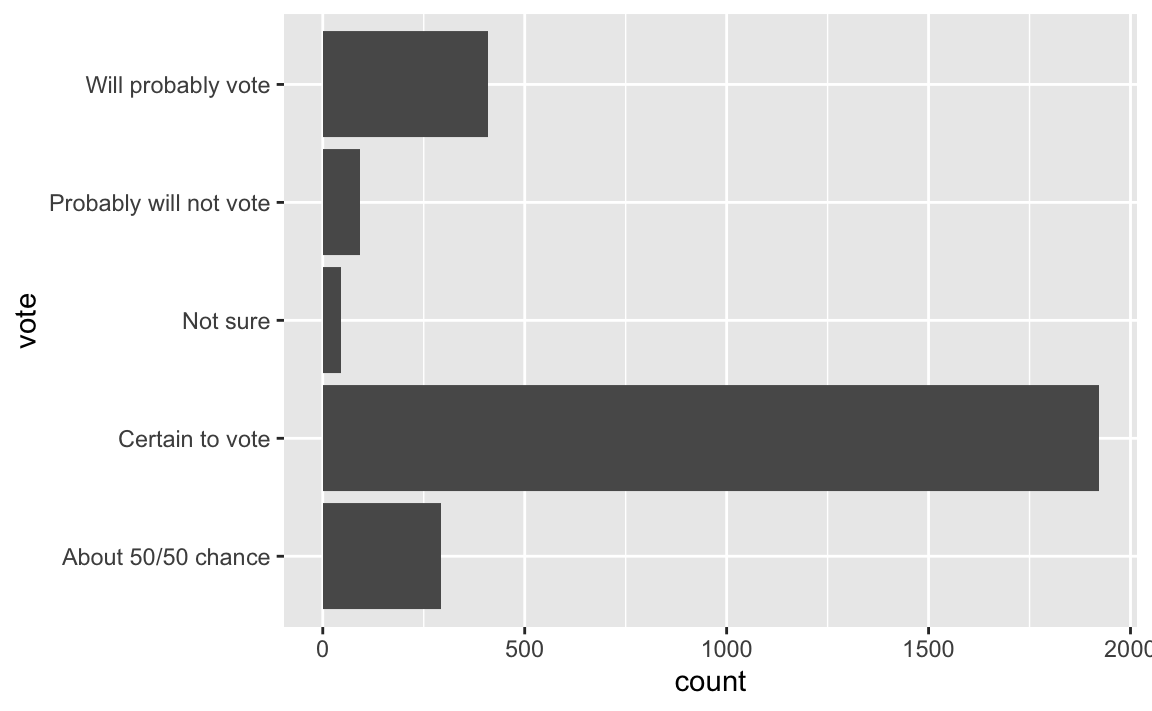
# Part 3

voting_survey |>
  count(vote) |>
  mutate(props = n / sum(n))
# A tibble: 5 × 3
vote n props
<chr> <int> <dbl>
1 About 50/50 chance 293 0.106
2 Certain to vote 1921 0.696
3 Not sure 44 0.0159
4 Probably will not vote 92 0.0333
5 Will probably vote 409 0.148 Task 2
Based on these data, we want to estimate the true proportion of registered US voters who are certain to vote in the next presidential election. Use the bootstrap to approximate a 95% confidence interval for this quantity.
# Prepare the data for analysis (pre-processing)

voting_survey <- voting_survey |>
  mutate(vote = if_else(
                        vote == "Certain to vote",
                        "Certain to vote",
                        "Not certain to vote")
         )

set.seed(20)

boot_dist <- voting_survey |>
  specify(response = vote, success = "Certain to vote") |>
  generate(reps = 1000, type = "bootstrap") |>
  calculate(stat = "prop")

ci <- boot_dist |>
  get_ci()
ci
# A tibble: 1 × 2
lower_ci upper_ci
<dbl> <dbl>
1 0.679 0.714visualize(boot_dist) +
shade_ci(ci)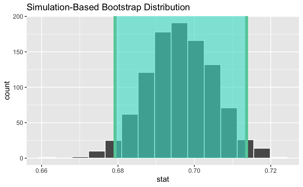
Task 3
BAD: “There is a 95% probability that the true proportion is between 67.9% and 71.4%.”
NOT SO BAD: “95% of the time, the true proportion is between 67.9% and 71.4%.”
CORRECT, BUT SHADY: “We are 95% confident that the true proportion is between 67.9% and 71.4%.”
Correct: “95% of the time, an interval constructed like this one will contain the true proportion.”
Task 4
Pew says that 66% of eligible US voters turned out for the 2020 presidential election. A newspaper claims that even more people will turnout in 2024, and cites this survey as evidence. Do these data provide convincing evidence for this claim?
Do two things:
- state the hypotheses
p = proportion of voters that turn out in 2024
H_0: p = 0.66
H_1: p > 0.66
One-sided test
- conduct a randomization test, at 5% discernability level. What is the conclusion of the test?
obs_stat <- voting_survey |>
    specify(response = vote, success = "Certain to vote") |>
    calculate(stat = "prop")

set.seed(525600)

null_dist <- voting_survey |>
  specify(response = vote, success = "Certain to vote") |>
  hypothesize(null = "point", p = 0.66) |>
  generate(reps = 1000, type = "draw") |>
  calculate(stat = "prop")

null_dist |>
  get_p_value(obs_stat, direction = "greater")
Warning: Please be cautious in reporting a p-value of 0. This result is an approximation
based on the number of `reps` chosen in the `generate()` step.
ℹ See `get_p_value()` (`?infer::get_p_value()`) for more information.# A tibble: 1 × 1
p_value
<dbl>
1 0Task 5
“There is a 0% chance that the null is true.”
“If the null were true, there is a 0% chance of seeing data like what we saw.”