Weights of books

Today we’ll explore the question “How do volume and weights books relate?” and “How, if at all, does that change when we take whether the book is hardback or paperback into consideration?”

Goals

• Build, fit, and interpret linear models with more than one predictor

• Use categorical variables as a predictor in a model

Packages

library(tidyverse)
library(tidymodels)
library(DAAG)

Data

The data for this application exercise comes from the allbacks dataset in the DAAG package. The dataset has 15 observations and 4 columns. Each observation represents a book. Note that volume is measured in cubic centimeters and weight is measured in grams. More information on the dataset can be found in the documentation for allbacks, with ?allbacks.

Single predictor

Plot the best fit line

Visualize the relationship between volume (on the x-axis) and weight (on the y-axis). Overlay the line of best fit. Describe the relationship between these variables.

ggplot(allbacks, aes(x = volume, y = weight)) +
  geom_point() +
  geom_smooth(method = "lm", se = FALSE) +
  labs(
    x = "Volume (cubic centimeters)",
    y = "Weight (grams)"
  )

`geom_smooth()` using formula = 'y ~ x'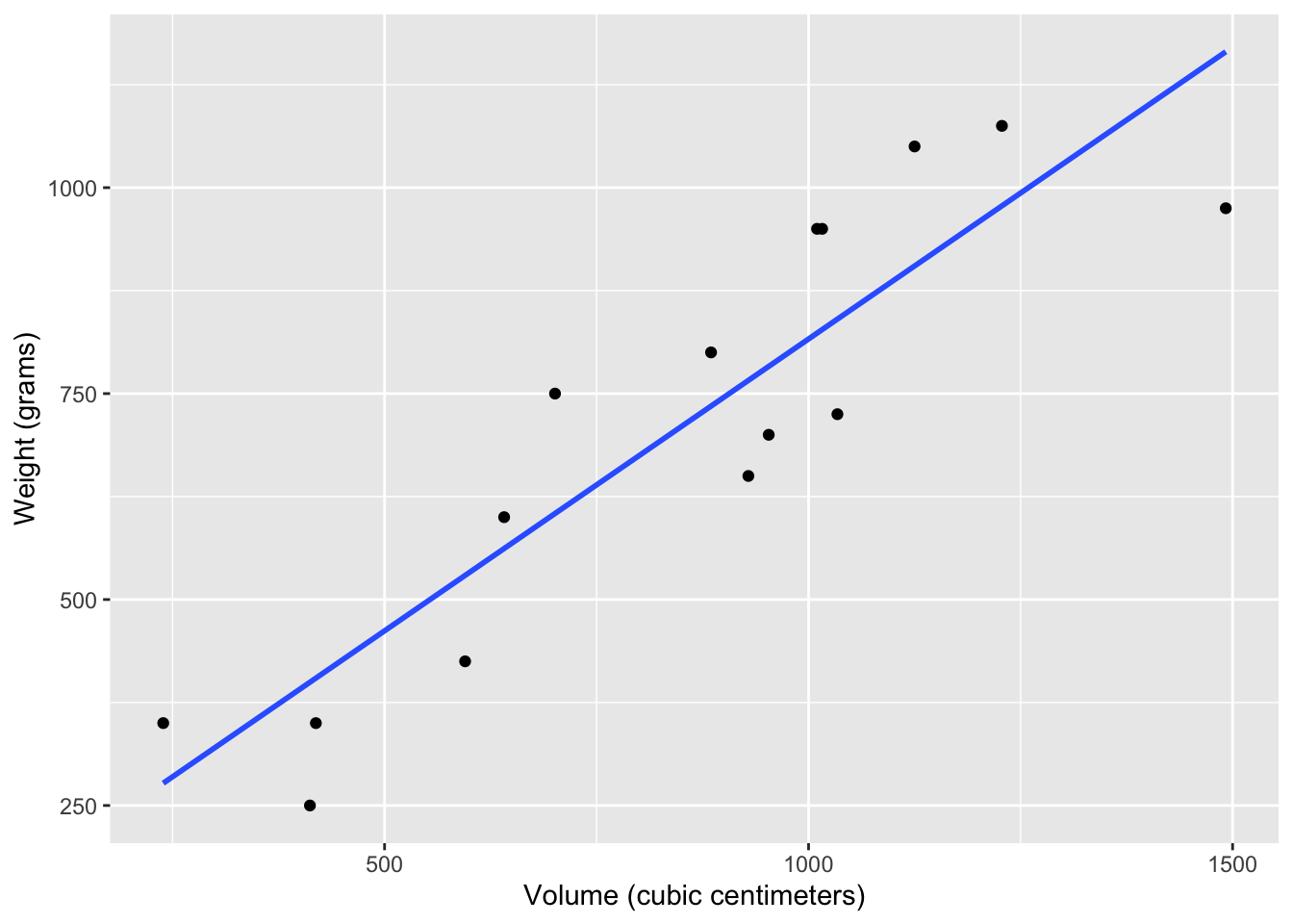

Add response here.

Get the estimated regression coefficients

Fit a model predicting weight from volume for these books and save it as weight_fit. Display a tidy output of the model.

weight_fit <- linear_reg() |>
  fit(weight ~ volume, data = allbacks)

tidy(weight_fit)

# A tibble: 2 × 5
  term        estimate std.error statistic    p.value
  <chr>          <dbl>     <dbl>     <dbl>      <dbl>
1 (Intercept)  108.      88.4         1.22 0.245     
2 volume         0.709    0.0975      7.27 0.00000626

Multiple predictors

Plot the best fit line(s)

Visualize the relationship between volume (on the x-axis) and weight (on the y-axis), taking into consideration the cover type of the book. Use different colors and shapes for hardback and paperback books. Also use different colors for lines of best fit for the two types of books. In addition, add the overall line of best fit (from Exercise 1) as a gray dashed line so that you can see the difference between the lines when considering and not considering cover type.

ggplot(allbacks, aes(x = volume, y = weight)) +
  geom_smooth(method = "lm", se = FALSE, color = "gray", linetype = "dashed") +
  geom_point() +
  labs(
    x = "Volume (cubic centimeters)",
    y = "Weight (grams)",
    shape = "Cover", color = "Cover"
  )

`geom_smooth()` using formula = 'y ~ x'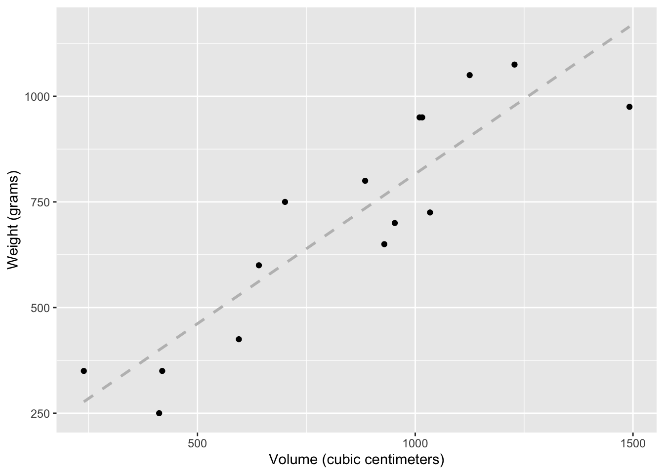

Get the estimated regression coefficients

Fit a model predicting weight from volume for these books and save it as weight_cover_fit. Display a tidy output of the model.

weight_cover_fit <- linear_reg() |>
  fit(weight ~ volume, data = allbacks)

tidy(weight_cover_fit)

# A tibble: 2 × 5
  term        estimate std.error statistic    p.value
  <chr>          <dbl>     <dbl>     <dbl>      <dbl>
1 (Intercept)  108.      88.4         1.22 0.245     
2 volume         0.709    0.0975      7.27 0.00000626

Prediction

Using the model you chose, predict the weight of a hardcover book that is 1000 cubic centimeters (that is, roughly 25 centimeters in length, 20 centimeters in width, and 2 centimeters in height/thickness).

new_book <- tibble(
  cover = "hb",
  volume = 1000
)

predict(weight_cover_fit, new_data = new_book)

# A tibble: 1 × 1
  .pred
  <dbl>
1  816.